Potential and Scientific Requirements of Optical Clock Networks for
Validating Satellite Gravity Missions

Stefan Schröder

Simon Stellmer

Jürgen Kusche

Session G4.1

Modern Concepts for Gravimetric Earth Observation

Fri, 30 Apr, 09:00–10:30 (CEST)

Use space, shift + space or the arrow keys to navigate through the slides.

Or press ESC for a slide overview.

Unless specified otherwise, the content of this side is licensed under a CC BY 4.0 license.

Goals of this presentation

Assess required measurement uncertainty of clock comparisons over Europe to sense non-tidal, time-variable gravity field changes
Discuss the spatial and temporal scales at which validation of existing time-variable gravity field data (GRACE/-FO) can be accomplished

Why validate?

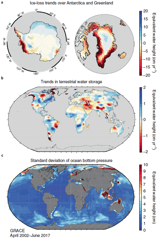
Since 2002 GRACE/-Follow-On observe the Earth's gravity field variations with unprecedented accuracy

identify/understand possible problems in sensor system and data analysis
better understand/quantify/calibrate GRACE error estimates
understand resolution limits of GRACE

Tapley et al. (2019)

How to validate?

...with ground measurement tools

Main problems:

GNSS comparison to GRACE requires an elastic loading model of the Earth
short wavelength signals like local groundwater discharge and recharge
affect the GNSS but does not follow elastic loading theory, i.e. can not be detected with GRACE

GNSS

Superconducting

Gravimeters

Main problem:

Local hydrology and wet air mass affect the gravimeters, but not GRACE; they are hard to model

If and how Superconducting Gravimeters (SG) can be used for GRACE validation is disputed (see e.g. the discussion between Van Camp et al., 2014 and Crossley et al., 2014)

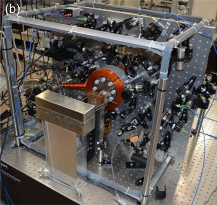
Optical clocks

Takamoto et al. (2015)

BKG

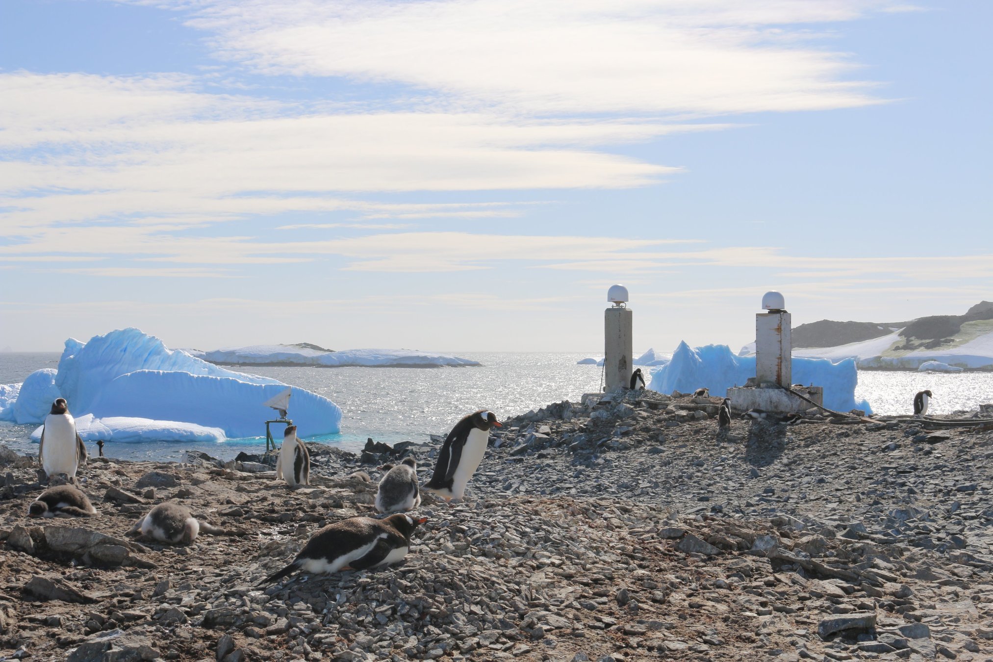
iGRAV043. Photo: Basem Elsaka, Uni Bonn

... will soon be a third ground measurement tool for GRACE validation

What do we measure with clocks?

\frac{\Delta f}{f} = \frac{\Delta U}{c²} = \frac{U_2 - U_1}{c²}

\frac{\Delta f}{f}

relative frequency difference, e.g. between two clocks*

\Delta U

gravity potential difference

speed of light

\frac{\Delta f}{f} = \frac{\Delta U}{c²} = \frac{U_2 - U_1}{c²}

\frac{\Delta f}{f}

relative frequency difference, e.g. between two clocks*

\Delta U

gravity potential difference

speed of light

*High performance optical clock comparisons over continental distances can be conducted via fibre links, e.g. with bidirectional amplifiers along the fibre link.

Lisdat et al. (2016)

The relative frequency difference is measured by comparing two clocks' frequencies
The gravity potential difference is easily deduced from that

We want to know the time-variable component of the gravity potential

\frac{\Delta f}{f} = \frac{\Delta U}{c²} = \frac{U_2 - U_1}{c²}

\frac{\delta f}{f} = \frac{\delta U}{c²} = \frac{\delta N - \delta h}{c²} \frac{GM}{R}

\delta N

geoid height change at the clock's location

\delta h

vertical displacement of the clock

\delta N - \delta h

would thus be the physical height change of the clock

\frac{\delta f}{f} = \frac{\delta U}{c²} = \frac{\delta N - \delta h}{c²} \frac{GM}{R}

\frac{\delta f}{f} = 10^{-18}

\delta N - \delta h = 0.9 \ \textrm{cm}

\frac{\delta f}{f} = 10^{-19}

\delta N - \delta h = 0.9\ \textrm{mm}

...

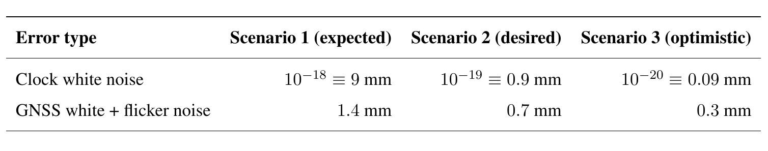
Sensitivity needed to observe non-tidal gravity changes over Europe (Goal 1)

RMS variability of non-tidal effects

Hydrology (CLM)

Atmophere (ERA-5 forced)

Glaciers (OGGM)

Corresponding time-series

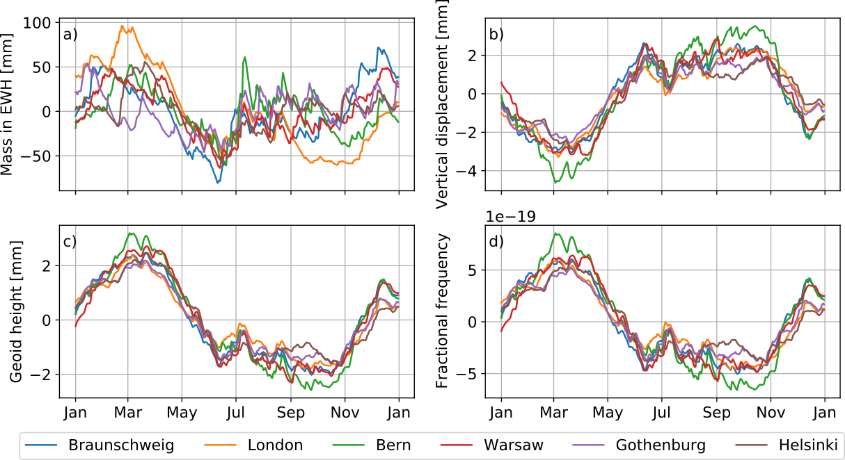
Hydrology

Atmosphere

Annual amplitudes in fractional frequency reach from the atmosphere and from hydrology
Interannual signals stronger from the atmosphere as well
However, signals acting on both clocks being compared cancel out, so let us focus on the difference between time series

8\times 10^{-19}

3\times 10^{-18}

Hydrology. All time series relative to the fractional frequencies in Braunschweig, Germany

annual amplitude only a third compared to the absolute signal
amplitude spectrum (b): already at monthly periods, the signal is too small to sense it with ' clocks' (Scenario 2)

10^{-19}

Atmosphere. All time series relative to the fractional frequencies in Braunschweig, Germany

signals up to approximately biweekly frequency (~100/yr) should be visible with ' clocks'

10^{-19}

Take Home

Non-tidal mass change effects will be visible in pan-European clock comparisons at the level

10^{-18}

... dependent on the observation duration
too be able to observe more than just some seasonal hydrological signal or very strong high/low-pressure fields, better clocks are needed

But how do the clocks compare to satellite gravity data and at which spatial scales can they be used for validation?

Spatial and temporal scales for satellite gravity field data validation (Goal 2)

sensitivity of the clock network 'overtakes' GRACE sensitivity eventually when increasing the spatial resolution
around these overtaking points, clock comparison data can be used to complement and validate GRACE data
Scenario 2: GRACE and the clock network show a similar sensitivity at 300 km resolution
at this resolution GRACE data becomes uncertain/dubious and here, a clock network with sufficiently dense clock distribution would be
important

at the daily to weekly scale, the clock comparisons would add additional information beyond the GRACE temporal resolution

Take Home

A sufficiently dense network of clocks with fractional frequency uncertainty can be used to validate satellite gravity data at the crucial resolution of 300 km and below

\bm{10^{-19}}